2.4. Extension and Application of Gradient Descent Based Algorithms

In this section, we present several examples to extend the concepts introduced so far. The section is divided into two parts. The first part highlights practical extensions of the gradient descent algorithm, by introducing a wider class of algorithm called first-order algorithms. The second part provides a more detailed case study demonstrating how gradient descent can be applied in practice.

2.4.1. First-Order Algorithms Beyond Gradient Descent

2.4.2. Example: Logistic Regression

In this section, we present a detailed case study applying gradient descent to solve a logistic regression (LR) problem. This example illustrates how the optimization techniques introduced earlier can be applied to real-world machine learning tasks and it will also help us understand practical algorithm behaviors. We will focus on key issues that may arise during the optimization process, and demonstrate how the theory developed so far can help resolve these challenges and provide practical insights.

2.4.2.1. Problem Setup

We are given a binary classification task with input-label pairs \((\vx_i, y_i)\) where \(\vx_i \in \RR^d\) and \(y_i \in \{-1, +1\}\). The logistic regression model aims to estimate the conditional probability that a data point belongs to the positive class:

\[ P(y_i = 1 \mid \vx_i) = h_\vw(\vx_i) := \frac{1}{1 + \exp(-\vw^\top \vx_i)}. \]

Here, \(\vw \in \RR^d\) is the vector of parameters to be learned. This model uses the logistic (sigmoid) function:

\[ \theta(s) = \frac{1}{1 + \exp(-s)}. \]

This prediction function can be compactly expressed for any label using:

\[ P(y_i \mid \vx_i) = \theta(y_i \cdot \vw^\top \vx_i). \]

To estimate \(\vw\), we minimize the empirical logistic loss:

(2.5)\[L(\vw) = \frac{1}{n} \sum_{i=1}^n \log\left(1 + \exp(-y_i \vw^\top \vx_i)\right).\]

This function is convex, differentiable, and commonly used in binary classification tasks. The key point is that \(L(\vw)\) penalizes the model when \(y_i \vw^\top \vx_i\) is small (i.e., when the margin is small or negative).

2.4.2.2. Gradient Descent Algorithm

We now apply gradient descent to minimize the loss function in Equation (2.5). The gradient is given by:

\[\nabla L(\vw) = -\frac{1}{n} \sum_{i=1}^n \frac{y_i \vx_i}{1 + \exp(y_i \vw^\top \vx_i)}.\]

Thus, the update rule at iteration \(r\) becomes:

\[\vw^{(r+1)} = \vw^{(r)} - \alpha \nabla L(\vw^{(r)}),\]

where \(\alpha > 0\) is the step size (learning rate).

2.4.2.3. One-Dimensional Example

To better visualize the optimization dynamics, consider a 1-dimension example where the optimization variable \(w\) is a scalar. Consider a problem with two data points:

• data point 1: \(x_1 = 1, \quad y_1 = +1\)

• data point 2: \(x_2 = 2, \quad y_2 = -1\)

Letting \(w \in \RR\) be the scalar weight (since \(d = 1\)), the loss becomes:

\[L(w) = \frac{1}{2} \log(1 + \exp(-w)) + \frac{1}{2} \log(1 + \exp(2w)).\]

This is a univariate convex function. Its gradient is:

\[\nabla L(w) = -\frac{1}{2} \cdot \frac{1}{1 + \exp(w)} + \frac{1}{2} \cdot \frac{2}{1 + \exp(-2w)}.\]

Gradient descent proceeds via:

\[w^{(r+1)} = w^{(r)} - \alpha \nabla L(w^{(r)}).\]

We can simulate this numerically or plot the function and its iterates to illustrate the convergence behavior.

import numpy as np
import matplotlib.pyplot as plt

# Logistic loss and its gradient
def logistic_loss(w):
    return 0.5 * np.log(1 + np.exp(-w)) + 0.5 * np.log(1 + np.exp(2 * w))

def logistic_grad(w):
    term1 = -0.5 / (1 + np.exp(w))
    term2 = 0.5 * 2 / (1 + np.exp(-2 * w))
    return term1 + term2

# Gradient descent parameters
alpha = 0.1      # step size
w0 = 0.0         # initial point
num_iters = 20   # number of iterations

# Store iterates
w_vals = [w0]
loss_vals = [logistic_loss(w0)]

# Run gradient descent
w = w0
for _ in range(num_iters):
    grad = logistic_grad(w)
    w = w - alpha * grad
    w_vals.append(w)
    loss_vals.append(logistic_loss(w))

# Plotting
w_grid = np.linspace(-3, 3, 300)
loss_grid = [logistic_loss(wi) for wi in w_grid]

plt.figure(figsize=(8, 5))
plt.plot(w_grid, loss_grid, label="Logistic Loss", linewidth=2)
plt.plot(w_vals, loss_vals, 'ro--', label="GD Iterates")
plt.xlabel("$w$")
plt.ylabel("$L(w)$")
plt.title("Gradient Descent on Logistic Regression (1D)")
plt.legend()
plt.grid(True)
plt.show()

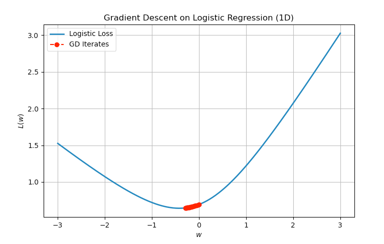
Fig. 2.2 Iteration for applying GD to the logistic regression problem with non-separable data points.

2.4.2.4. Behavior Under Linearly Separable Data

An interesting phenomenon arises when the dataset is linearly separable — that is, when there exists a vector \( \vw \) such that:

\[ y_i (\vw^\top \vx_i) > 0 \quad \text{for all } i. \]

In this case, the empirical logistic loss:

\[ L(\vw) = \frac{1}{n} \sum_{i=1}^n \log(1 + \exp(-y_i \vw^\top \vx_i)) \]

has no finite minimizer. The loss can be made arbitrarily small by increasing the magnitude of \( \|\vw\| \), while maintaining the sign of \( y_i \vw^\top \vx_i \).

Proposition: No Finite Minimizer Under Linear Separability

If the dataset is linearly separable, then the logistic loss satisfies:

\[ \inf_{\vw \in \mathbb{R}^d} L(\vw) = 0, \]

but the infimum is not attained by any finite \( \vw \).

To better understand the behavior of gradient descent under linearly separable data, we revisit a simple 1D example with the following data point:

• data point 1: \(x_1 = -1\), \(y_1 = +1\)

• data point 2: \(x_2 = +1\), \(y_2 = -1\)

Let \(w \in \mathbb{R}\) be the scalar weight. The logistic regression loss becomes:

\[ L(w) = \frac{1}{2} \log\left(1 + \exp(w)\right) + \frac{1}{2} \log\left(1 + \exp(w)\right) = \log(1 + \exp(w)). \]

This is a linearly separable dataset in 1D: the classifier \(\text{sign}(w x)\) correctly classifies both points when \(w < 0\).

---

2.4.2.5. Gradient and Gradient Descent Update

The derivative of the logistic loss is:

\[ \nabla L(w) = \frac{\exp(w)}{1 + \exp(w)} = \frac{1}{1 + \exp(-w)} = \theta(w), \]

where \(\theta(\cdot)\) is the sigmoid function.

Gradient descent proceeds as:

\[ w^{(r+1)} = w^{(r)} - \alpha \cdot \theta(w^{(r)}). \]

We simulate the algorithm below and observe the monotonic decrease of the loss and divergence of the iterates.

import numpy as np
import matplotlib.pyplot as plt

# Logistic loss and gradient for separable case
def logistic_loss(w):
    return np.log(1 + np.exp(w))

def logistic_grad(w):
    return 1 / (1 + np.exp(-w))  # sigmoid(w)

# Gradient descent settings
alpha = 0.1
w0 = 0.0
num_iters = 30

# Store iterates
w_vals = [w0]
loss_vals = [logistic_loss(w0)]

# Run gradient descent
w = w0
for _ in range(num_iters):
    grad = logistic_grad(w)
    w = w - alpha * grad
    w_vals.append(w)
    loss_vals.append(logistic_loss(w))

# Plotting
w_grid = np.linspace(-8, 2, 300)
loss_grid = [logistic_loss(wi) for wi in w_grid]

plt.figure(figsize=(8, 5))
plt.plot(w_grid, loss_grid, label="Logistic Loss", linewidth=2)
plt.plot(w_vals, loss_vals, 'ro--', label="GD Iterates")
plt.xlabel("$w$")
plt.ylabel("$L(w)$")
plt.title("Gradient Descent on Separable 1D Logistic Regression")
plt.legend()
plt.grid(True)
plt.show()

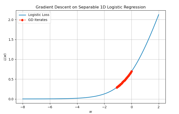
Fig. 2.3 Iteration for applying GD to the logistic regression problem with separable data points.

2.4.2.6. Logistic Regression with L2 Regularization

To address the issue of unbounded iterates in the linearly separable setting, and to improve generalization, we often add L2 regularization to the logistic regression loss:

\[ L_\lambda(\vw) = \frac{1}{n} \sum_{i=1}^n \log(1 + e^{-y_i \vw^\top \vx_i}) + \frac{\lambda}{2} \|\vw\|^2. \]

Here, \(\lambda > 0\) is the regularization parameter that balances the trade-off between minimizing training loss and controlling model complexity (via the norm of \(\vw\)).

---

The regularized Logistic Regression problem has the following properties:

• The function \(L_\lambda(\vw)\) is strongly convex if \(\lambda > 0\).

• The problem admits a unique global minimizer for all datasets (including linearly separable ones).

• The solution satisfies \(\|\vw_\lambda^*\| < \infty\).

• Gradient descent applied to \(L_\lambda(\vw)\) converges globally and at a linear rate (under smoothness assumptions).

In particular, the gradient of \(L_\lambda(\vw)\) is:

\[ \nabla L_\lambda(\vw) = -\frac{1}{n} \sum_{i=1}^n \frac{y_i \vx_i}{1 + e^{y_i \vw^\top \vx_i}} + \lambda \vw. \]

The regularization term \(\lambda \vw\) encourages smaller weight norms and stabilizes optimization.