4.1. SGD and its convergence#
The SGD method aims to tackle (4.1) by mimicking the gradient descent method applied on the stochastic optimization problem. In particular, observe that if we have \(\xi \sim {\cal D}\), then
Particularly, when conditioned on \(\vw\), the expected value of the right hand side equals the left hand side. The above insight motivates the SGD method as follows:
Algorithm 4.1 (Stochastic Gradient (SGD) Method)
Input: initial point \(\vw^0\), stepsize sequence \(\{ \eta_t \}_{t \geq 0}\), max. no. of iterations \(T\).
For \(t=0,1,2,..., T-1\),
Output: last iterate \(\vw^T\), or the solution sequence \(\{ \vw^t \}_{t=1}^T\).
Unlike the deterministic gradient method, the sequence \(\{ \vw^t \}_{t=1}^T\) generated by the SGD method is a random process itself (in fact, a Markov chain). As such, there are several subtleties in analyzing the convergence properties of the solution sequence. Here, the common forms of convergence are almost-sure convergence, convergence in expectation, etc. We will demonstrate the convergence in expectation of SGD under the simplest setting, i.e., with smooth (but possibly non-convex) objective function. Interested readers may refer to (ref.) for further discussions.
In addition to Assumption 2.1 on the expected objective function \(f(\vw)\), we need the following condition on the stochastic gradient:
Assumption 4.1 (Stochastic Oracle)
There exists \(\sigma \geq 0\) such that for any \(\vw \in \mathbb{R}^d\), we have
In other words, the stochastic oracle used in the SGD method is both unbiased and has bounded variance.
We observe the following convergence in expecatation result:
Theorem 4.1 (Convergence of SGD Method (Smooth Case))
Under Assumption 2.1, Assumption 4.1 and suppose that the step size satisfies \(\eta_t \leq 1/L\). For any \(T \geq 1\), the following holds:
Proof (SGD for Smooth Objective Function)
The proof is very similar to that of Theorem 2.6. Observing that under Assumption 2.1, it holds for any \(t \geq 0\) that,
By noting that \(\vw^{t+1} - \vw^t = - \eta_t \nabla \ell (\vw^t; \xi_{t})\), we have
We denote \({\cal F}_k\) as the filtration of the random variables \(\{ \vw^0, \xi^1, \ldots, \xi^{t-1}, \vw^t \}\). Under Assumption 4.1, we have the following conditional expectations:
and
Taking the full expectation on both sides of (4.3) yields
Using \(\eta_t \leq 1/L\) simplifies the above to
This implies
Summing both sides from \(k=0\) to \(k=K-1\) yields the desired result.
From the results in Theorem 4.1, we notice that if we set \(\eta_t = 1 / \sqrt{t}\) (to make \(\eta_t \leq 1/L\), we could take \(\eta_t = 1 / (\sqrt{t}L)\)) for all \(t=0,...,T-1\), then for sufficiently large \(T\), one has
Also if we take \(\eta_t = 1 / \sqrt{T}\) for all \(t=0,...,T-1\), we have
These results show that the convergence (in expectation) to stationary points for the SGD method.
4.1.1. A simple example of running SGD in PyTorch#
In the following code blocks, we use SGD to train the Cifar10 dataset on ResNet. Torch has a module torch.optim which can help you load the SGD optimizer directly. You can change torch.optim.SGD to torch.optim.Adagrad, torch.optim.RMSprop or torch.optim.AdamW to see the effect of different optimizers.
# Simple Pytorch Training script for Image Classification (Resnet18 model on CIFAR10 dataset) using SGD

import torch
import torch.nn.functional as F
from torchvision import datasets, transforms
from torch.autograd import Variable
from torchvision.models import resnet18

import matplotlib.pyplot as plt

device = 'cuda' if torch.cuda.is_available() else 'cpu'

# typical augmentation for CIFAR
transform_train = transforms.Compose([
    transforms.RandomCrop(32, padding=4),
    transforms.RandomHorizontalFlip(),
    transforms.ToTensor(),
    transforms.Normalize((0.4914, 0.4822, 0.4465), (0.2023, 0.1994, 0.2010)),
])

transform_test = transforms.Compose([
    transforms.ToTensor(),
    transforms.Normalize((0.4914, 0.4822, 0.4465), (0.2023, 0.1994, 0.2010)),
])


trainset = datasets.CIFAR10(root='./data', train=True, download=True, transform=transform_train)
testset = datasets.CIFAR10(root='./data', train=False, download=True, transform=transform_test)
nclasses = 10 # CIFAR10 has 10 classes

batch_size = 128
epochs = 10

train_loader = torch.utils.data.DataLoader(trainset, batch_size=batch_size, shuffle=True, num_workers=8)
test_loader = torch.utils.data.DataLoader(testset, batch_size=batch_size, shuffle=False, num_workers=8)

model = resnet18(num_classes=nclasses)
model.to(device)

optimizer = torch.optim.SGD(model.parameters(), lr=0.1, momentum=0.9, weight_decay=5e-4)
scheduler = torch.optim.lr_scheduler.CosineAnnealingWarmRestarts(optimizer, epochs, T_mult=1)


def train(epoch, train_loader, model, optimizer, scheduler):
    nbatches = len(train_loader)
    running_loss = 0
    model.train()
    for batch_idx, (data, target) in enumerate(train_loader):

        data, target = data.to(device), target.to(device)
        data, target = Variable(data), Variable(target)
        optimizer.zero_grad()

        output = model(data)
        loss = F.cross_entropy(output, target)

        loss.backward()
        torch.nn.utils.clip_grad_norm_(model.parameters(), 3)
        optimizer.step()

        scheduler.step((epoch-1) + batch_idx/nbatches )
        running_loss += loss.item() * data.size(0)

    epoch_loss = running_loss / len(train_loader.dataset)
    print(f'Epoch: {epoch} \tLoss: {epoch_loss}')
    return epoch_loss


def test(epoch, test_loader, model):
    model.eval()
    test_loss = 0
    correct = 0
    for data, target in test_loader:

        data, target = data.to(device), target.to(device)
        data, target = Variable(data), Variable(target)
        output = model(data)
        test_loss += F.cross_entropy(output, target, reduction='sum').item()
        pred = output.data.max(1, keepdim=True)[1]
        correct += pred.eq(target.data.view_as(pred)).long().cpu().sum()

    test_loss /= len(test_loader.dataset)
    print('\n({}) - Test set: Average loss: {:.4f}, Accuracy: {}/{} ({:.2f}%)\n'.format(
        epoch, test_loss, correct, len(test_loader.dataset),
        100. * correct / len(test_loader.dataset)))
    return test_loss, 100. * correct / len(test_loader.dataset)

train_losses = []
test_losses = []
test_accs = []
for epoch in range(1, epochs + 1):

    train_loss = train(epoch, train_loader, model, optimizer, scheduler)

    if epoch % 1 == 0:
        test_loss, test_acc = test(epoch, test_loader, model)

    train_losses.append(train_loss)
    test_losses.append(test_loss)
    test_accs.append(test_acc)
Downloading https://www.cs.toronto.edu/~kriz/cifar-10-python.tar.gz to ./data/cifar-10-python.tar.gz
100%|██████████| 170498071/170498071 [00:07<00:00, 22756360.38it/s]
Extracting ./data/cifar-10-python.tar.gz to ./data
Files already downloaded and verified
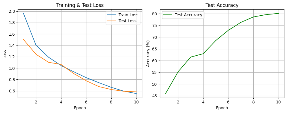
Epoch: 1 Loss: 1.9615433359909058
(1) - Test set: Average loss: 1.5024, Accuracy: 4596/10000 (45.96%)
Epoch: 2 Loss: 1.40224799369812
(2) - Test set: Average loss: 1.2430, Accuracy: 5525/10000 (55.25%)
Epoch: 3 Loss: 1.1913091995429992
(3) - Test set: Average loss: 1.1020, Accuracy: 6149/10000 (61.49%)
Epoch: 4 Loss: 1.044463742198944
(4) - Test set: Average loss: 1.0641, Accuracy: 6293/10000 (62.93%)
Epoch: 5 Loss: 0.936025900554657
(5) - Test set: Average loss: 0.9054, Accuracy: 6854/10000 (68.54%)
Epoch: 6 Loss: 0.8328752424430848
(6) - Test set: Average loss: 0.7783, Accuracy: 7290/10000 (72.90%)
Epoch: 7 Loss: 0.7448515315628051
(7) - Test set: Average loss: 0.6759, Accuracy: 7628/10000 (76.28%)
Epoch: 8 Loss: 0.6620122916030884
(8) - Test set: Average loss: 0.6234, Accuracy: 7860/10000 (78.60%)
Epoch: 9 Loss: 0.5950784549331665
(9) - Test set: Average loss: 0.5929, Accuracy: 7958/10000 (79.58%)
Epoch: 10 Loss: 0.5526298828697205
(10) - Test set: Average loss: 0.5829, Accuracy: 8012/10000 (80.12%)
# Plot the results
epochs_range = range(1, epochs + 1)

plt.figure(figsize=(10,4))

# Plot both losses on the same plot
plt.subplot(1, 2, 1)
plt.plot(epochs_range, train_losses, label='Train Loss')
plt.plot(epochs_range, test_losses, label='Test Loss')
plt.xlabel('Epoch')
plt.ylabel('Loss')
plt.title('Training & Test Loss')
plt.grid(True)
plt.legend()

# Plot test accuracy
plt.subplot(1, 2, 2)
plt.plot(epochs_range, test_accs, label='Test Accuracy', color='green')
plt.xlabel('Epoch')
plt.ylabel('Accuracy (%)')
plt.title('Test Accuracy')
plt.grid(True)
plt.legend()

plt.tight_layout()
plt.show()